SimpleGeo Solid Modeler - 4.3
(c) Copyright 2004 - 2011 Chris Theis, Karl Heinz Buchegger
|
Reference nodes
Layers and visibility
Materials
Merging
Biasing wizardParametric modeling & scripting language
Export to FLUKA
Export to PHITS
Camera
Zoom
Identifying objects
Measuring distances in 2D & 3D
DaVis3D (data averaging, visualization & extraction)PCloud3D (particle position & direction visualization + some statistical analysis)
PipsiCAD3D (track visualization & animation)
![]() Frequently
Asked Questions (FAQ)
Frequently
Asked Questions (FAQ)
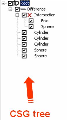
Creation of a boolean tree |
Basic primitives ![]() & boolean
operators
& boolean
operators ![]() are created via
the toolbar or the menu. They are automatically inserted as children of the
currently active hierarchy
node in
the tree-view on the left.
If the currently selected node is for example a
union the
new object will be a child of the union. In case that the currently selected
object is a primitive then
the newly created object will be inserted as a sibling!
are created via
the toolbar or the menu. They are automatically inserted as children of the
currently active hierarchy
node in
the tree-view on the left.
If the currently selected node is for example a
union the
new object will be a child of the union. In case that the currently selected
object is a primitive then
the newly created object will be inserted as a sibling!
 Of
course the order & thus the actual
boolean tree can be modified. This is done by simply
dragging & dropping a primitive/operator onto another hierarchy node.
To modify the order of the subnodes one can simply select a subnode and drop
it on the parent node, which will result in the insertion of the selected
subnode at the end.
Of
course the order & thus the actual
boolean tree can be modified. This is done by simply
dragging & dropping a primitive/operator onto another hierarchy node.
To modify the order of the subnodes one can simply select a subnode and drop
it on the parent node, which will result in the insertion of the selected
subnode at the end.
Boolean operators are
indicated in the tree with an icon in order to determine their type after
the initial name
has been changed. Furthermore, their type is indicated in the property bar
on the right side of the screen.
Attention: As a rule for the
difference operator one has to keep in mind that the first child is
the primitive that is subtracted from!!
As a default the boolean CSG tree is re-evaluated
every time a property of a node or the
hierarchy itself is changed. This can become a time wasting task when a lot
of properties
are changed. Thus the automatic update can be temporarily disabled/enabled
by clicking on the
gearwheel button ![]() on the toolbar.
on the toolbar.
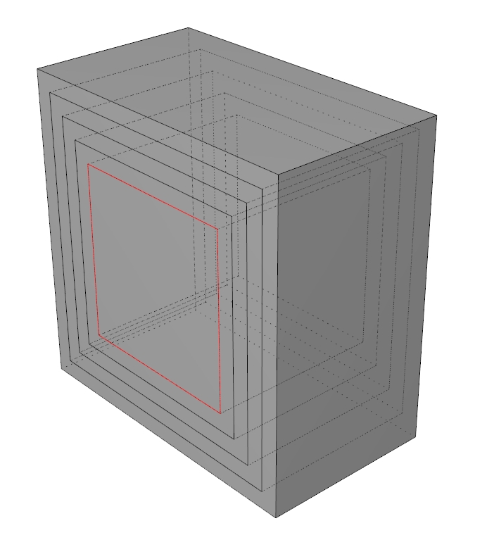
It is possible to change the type of a boolean operator node by selecting it and pressing the right mouse button. Consequently a context menu offers to change the type.
Figure 1: Example of a CSG tree
All modeling actions (add, delete, change
property, change of hierarchy) are now managed via an
undo manager. Hence, they can be undone or redone. A log is kept of the last
40 commands
which can be undone sequentially at once. Please be aware that actions that
affect the visibility are not linked into the undo queue as they would easily
clog the queue and overwrite actions that are probably more important to be
available for an undo operation.
Property fields |
Starting with version 3.1 the numerical edit fields, e.g. position/rotation/size etc., can evaluate mathematical expressions. If for example the value 213.5 is the current value of the X-position then it is possible to enter 213.5 + 36.231 which will be evaluated after the ENTER key has been pressed. The following functions are available:
mathematical operators + - * / ^
parentheses (){}, nested in arbitrary levels
mathematical functions: SQRT, "power of" using the ^ operator
binary operators AND & and OR |
relation operators =, <, >, <>, <=, >=
Hint: This functionality is usually supported strictly for numerical fields. However, it is also available for the IMPORTANCE property!
Relative coordinate frames |
As a general approach relative coordinate
systems are used. Not only objects but also
boolean operators are identified with a position and rotation. The used values
are
not absolute ones but relate to then ones already specified by a superior hierarchy
node!
Consequently the translation/rotation of whole geometry parts or even geometries
can easily
be performed by changing the position/rotation of a superior hierarchy node
without the need
to adjust the settings for each primitive.
Still, the relative coordinate frames can be converted into absolute
coordinates of primitives by choosing the respective region and opening
the context
menu with the right mouse click and selecting "CSG
tree tools
-> Convert rel. to abs. positions". This option can be particularly
useful in case the user wants to use references to primitives of the respective
modified region. Otherwise it might be possible that for the rendering of references
the transformation matrix of the source primitive is not taken into account correctly,
and thus, the body might be drawn at an incorrect position. Please note that
for the export this does not affect the validity of the produced output. Still,
it might be disturbing and thus, it is recommended to convert absolute to relative
positions if it is planned to create references to constituents of a region which
uses relative coordinate frames.
Recursive cloning of nodes |
Selecting a node in the boolean tree (primitive or boolean operator) and pressing
Ctrl+C will
result in recursive cloning of the underlying tree branch. On-the-fly creation
of a clone
(also of whole sub-trees) is also possible by holding the Ctrl key while dragging
the sub-tree
to be cloned.
Creation of replicas |
Sometimes it might be useful to create replicas of whole entities in your geometry like the full model of a magnet. A simple copy is not possible as copying regions usually yields what is called "deep copies". That means that primitives are cloned but references will still point to the original source primitive and not to the cloned ones. For a replica the situation is somewhat different because one would like to have a copy of a whole entity which is totally independent from its source. In order to do this the user has to take the following steps:
1.) Drag and drop all regions which make up your entity, e.g. the magnet, in a group node.
2.) Select this group and create a copy either via Ctrl+C or via the context menu "Create replica from group".
As a consequence a new group is created which contains copies of the source primitives/regions and references which are relinked to the cloned primitives/regions instead of the original sources. The next step would be to translate/rotate the whole group to the new location by setting the position/rotation of the group node. All sub-nodes of the group will be automatically placed in relative coordinate frames with respect to the group's position. Once the final position is determined the user can, if requested, convert the relative coordinate frames to absolut positions via "CSG tree tools -> Convert rel. to abs. positions". Furthermore, grouped entities can be ungrouped via the context menu "Right mouse click --> CSG tree tools --> Ungroup group node".
Layers & visibility |
Layers (which are called groups in SimpleGeo) can be created
by using the boolean group operator ![]() from
the toolbar. A layer/group does not have a boolean meaning but represents only
a logical collection of nodes
and subnodes.
Every node can be enabled or disabled for the rendering process by selecting
it and pressing
Space or clicking on the checkbox
next to it. Please note that the
disabling and
enabling
acts recursively!Thus, it is good practice to enable/disable always the top-most
node.
from
the toolbar. A layer/group does not have a boolean meaning but represents only
a logical collection of nodes
and subnodes.
Every node can be enabled or disabled for the rendering process by selecting
it and pressing
Space or clicking on the checkbox
next to it. Please note that the
disabling and
enabling
acts recursively!Thus, it is good practice to enable/disable always the top-most
node.
Especially for large and complex geometries it is convenient to store the visibility state. This allows for the inspection of different objects and details without having to turn on and off the visibility manually every time. To store the visibility state = "snapshot" the user simply has to select the menu item "Macros -> Predefined scripts -> Save snapshot". Storing the current state in a buffer only can be achieved by selecting "Take snapshot". Please note that this buffer is not written to a file and is therefore only available during runtime.
The major functions are available from the toolbar ![]() .
.
Planes |
Mathematically planes are regarded as infinite half-spaces and infinity is something which does not work well with deterministic machines like computers. Therefore and due to the fact that infinite half-spaces might result in non-regularized and thus invalid boolean solids they are treated as limited planes (at least for visualization). A plane is indicated by a slightly transparent green (upper) and an opaque red side with an upwards pointing normal vector at the lower left corner.
As a general rule the upper part of a primitive intersected with a plane will remain!
In order to avoid confusion planes are only visible when
selected in the hierarchy tree
on the left. Naturally they can be used in an intersection to create an arbitrary
primitive
delimited by faces. In this case only the enclosed volume (meaning the volume
delimited by
planes with outward pointing normals!!) will be created. Consequently only
valid boolean
solids will be visible! If the created object is not rendered then there is
a problem with
the regularization and thus the boolean equation is not valid!
For the moment infinite half-spaces are not yet exported by the PovRay export filter.
Materials |
In principle there is a list of standard materials that are indexed via a (FLUKA) number. The selection of the material is done on a primitive basis and can be performed via the property dialog on the right side. The list can be extended using the Edit item of the Material menu. The dialog also allows for changing the rendering properties of a material. The assignment of the material is done via a drop-down box in the property view of the currently selected node. For regions that are made up of several primitives combined by Boolean operators, the material assignment must be made for the top-most node, which will be a Boolean operator. All sub-nodes will automatically show the identical material assignment in their properties. Any material assignment which is done for a sub-node that constitutes only a part of the region, does not affect the material assignment of the whole region!
Please note that if no existing material database is found a default file (material.db) is created in whatever directory the current scenery is created or loaded from.
Attention: The assignment of the materials in the exported FLUKA file is handled via the numerical index and not the name as FLUKA imposes limitations on the number of characters used and also case sensitivity.
Merging with other sceneries |
Using the Merge function found in the File menu allows for merging the current geometry with one loaded from a file. The merged geometry can be treated as a group and thus, manipulated as a group, or it can be split into its constituent regions. Both options will be presented to the user after the merge function has been executed. Please see also the section "creation of replicas" for some helpful information.
Biasing wizard |
Starting with version 4.2 two different biasing wizards are available to facilitate the creation of sub-regions that are usually required for geometric importance biasing. In order to activate one of them the user has to select the body/region which is to be modified and open the context menu with a right mouse-click. Under the menu item "Biasing wizard" the following options are available:
1.) Splitting wizard:
The currently selected body/region will be split into sub-regions. For this purpose the user has to specify the number of sub-regions that should be created, the direction and the splitting dimension of the sub-regions. Subsequently a number of planes are created that will be used to cut the original body/region into several new regions. The splitting dimension basically reflects the distance between these planes. All regions & bodies will be created automatically and importances can be assigned automatically if the users wishes. Specifying an importance of 1.4 will result in an importance 1.4 for the first new region, 1.4^2 for the second, 1.4^3 for the third etc.
Please note that the required planes & regions will be named automatically by reusing the name of the original body/region and appending a suffix. Some codes like FLUKA have a restriction of 8 characters for a name and might truncate longer names silently. Thus, names starting to be different at the 9th character or later will not be recognized as being different by such codes!!!
2.) Concentric regions:
Very often a user wishes to create biasing regions which are based on nested or concentric bodies. For example nested boxes with "growing" dimensions to the outside.
This can be easily achieved for boxes, cylinders and spheres using the concentric region wizard. As a first step the smallest source primitive (either box, cylinder or sphere) has to be created and the concentric region wizard has to be activated from the context menu with a right mouse click. Depending on the primitive type different parameters will be available to the user to influence the creation of the concentric regions. In case of a sphere only the radii can be set wherease radius & height are available for cylinders. For boxes all three axes can be set individually. As a consequence the user is not restricted to creating concentric cubes but has the free choice of symmetry.
The biasing wizard will create all primitives + a full region description of the requested structure. Optionally the assignment of importances is available in the same manner as in the splitting wizard.
Parametric modeling & scripting |
It is possible to create models or part of models using
a very simple macro scripting language.
Several of these macros can be stored in macro libraries which can be created
by the user.
The modeler supplies a macro editor with syntax coloring and basic features
like (select,
copy,paste and undo).
For a detailed description & examples of the scripting
language please refer to the
accompanying HTML file (macro_commands.htm).
A couple of predefined built-in scripts are supplied to increase or decrease the level-of-detail (LOD) for curved surfaces. Decreasing the LOD will result in faster building times of the geometry but naturally in less smooth surfaces. However, it should be noted that this has no influence on the geometry export for the Monte Carlo codes because there the analytic description of the bodies are used!!
Reference nodes |
Reference nodes are sometimes refered to as "geometry sharing" in computer graphics. Using textual input the user implicitely uses this because it is very convenient and trivial. However, as soon as one ventures into graphics triviality is quickly lost and thus, this requires a more in-depth explanation.
A very simple FLUKA input of regions could look like this:
001 +1 -2
002 +2
This means that in the first region primitive #2 is subtracted from primitive #1. However, the same primitive #2 is used to define a second region with a different material! Consequently the geometry of primitive #2 is shared. In the textual input this is simple as simple can be, but for visualization this becomes quite intricate. To visualize primitives/regions you need geometric information as well as material information and other attributes. In order to support geometry sharing a special node type named "Reference node" was implemented, which uses the same geometric information but overrides material and other attributes. In the example given above primitive #2 would be instantiated one time as the original primitive (source) and a second time as a reference (or referer) to the original. In order to allow for more flexibility it is not required that the first occurence is the source but it can also be a reference node. However, there must exist one original source node somewhere. This required a total rewrite and reimplementation of the geometry and render caching scheme, which is implemented in SimpleGeo for speed optimization. The new non-linear scheme is much more complex but it reduces the memory consumption by about 20% to 25% and especially for complex geometries the gain in speed is significant.
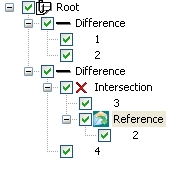
An example of references in SimpleGeo:
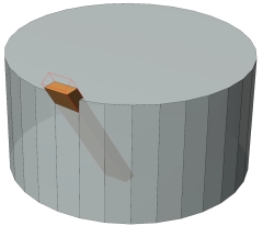
Figure 2 and Figure 3: Example geometry |
The example geometry in figure 2 basically consists of a cylinder of which a tilted brown slab is subtracted (region 1). This slab (primitive #2 as shown in figure 3) is delimited by an upper and a lower plane (region 2). The big advantage of reference nodes is that whenever you change the geometric properties of primitive #2 it will automatically be updated and effect all regions which this primitive/reference is used in. This example is included as Reference1.dat in the demo data files. You can simply try to change the parameters of the source slab to see that the affected regions are updated automatically.
|
ATTENTION: References should not be mistaken with copies/clones! In order to create a copy of a region/primitive one use the menu item "Clone" found under the "Edit" menu or simply press Ctrl + C. Consequently, a clone of the currently selected node is created which means that this is a newly instantiated node which is an exact copy of the source. Any changes DO NOT effect the previous source anymore. Keep in mind that you should immediately change the name of the copy because otherwise you will end up with multiple geometry definitions of a primitive sharing the same name! Depending on the Monte Carlo code used this will lead to crashes or ambiguous invalid geometry definitions running a simulation with the exported geometry. The FLUKA exporter in SimpleGeo tracks down this problem and will notify you, but you should try to avoid it in the first place because fixing the naming scheme in a large geometry can easily become a nightmarish experience.
How to create reference nodes:
Basically there are two different ways to create references to a source node. The first one is by selecting the source node and dragging it to the target region while keeping the Shift key pressed. Consequently, a reference node is created in the target region. This node can be identified as a reference because an envelope icon appears next to it, and it is prefixed with the string "R_".
The second way to create a reference is to use the right mouse button in the CSG tree to open the context menu. In the context menu you will find the respective item named "Create reference node", which creates an empty (!) reference. You can drag and drop this node like any other node, even if it is still empty. In order to assign a source node you simply have to select the respective source and drop it on the empty reference node.
By selecting the reference node you will get a special list of attributes that are available for references (see Figure 4).
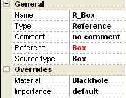
Figure 4: Examplatory attributes of a reference
As you can see from Figure 4 you cannot change any geometric parameters but only those that are overriden like the Material. All geometric parameters are taken from the original source node. However, the original source is available as a child of the reference node in the CSG tree and there you can apply any changes regarding the geometry. The source and all referers are automatically updated.
Finding all references to a source node:
If a node is referenced somewhere else this is indicated in the attribute list of the source node. In case you quickly need to find all references you can use the find dialog. Simply select the original node and press Ctrl + F or open the dialog via the menu "Edit" -> "Find". Do not type in any name but rather select "References" in the "Search in" combo box. This will find all references to the current source node and you can easily navigate forwards and backwards with the available buttons.
Export to FLUKA |
Using combinatorial solid geometries the same result can be obtained with different CSG tree representations. SimpleGeo uses what is called a "recursive CSG tree", which allows for subtracting whole regions from other regions for example. However, with FLUKA this has not been able until version 2005. With this version parentheses have been introduced which are internally re-written into what is called a "normalized tree form". This rewriting might produce a significant overhead in the geometry representation of which the user should be aware. At the moment there is work going on to optimize this process within FLUKA. In case that the "old" structures (even with names) are used FLUKA does not rewrite the tree internally and thus, no overhead is produced. Depending on your needs you might consider working without these recursive structures even if it is possible to use them in SimpleGeo.
The "old" structures that do not require recursion/parentheses imply the following rules:
Regions can be made up of intersections that may contain ONE difference and various single primitives, or differences that may contain ONE intersection and various single primitives:
Example1: +1 +2 +3 -5 -6 ...... this could be interpreted as (+1+2+3) -5 -6
Of course you can also use unions like before, but you should stay away of structures like intersections that contain differences that contain intersections etc.
To export geometry to FLUKA you simple have to select "File" -> "Export" -> "FLUKA...". In the dialog box you can choose different types. The first one labelled "FLUKA input file (*.inp)" will create an input file using the old fixed format syntax which requires numerical names! If the body identifiers are not of numerical type the export will be stopped. Via the menu item "Macros" -> "Predefined scripts" -> "Names" an automatic conversion algorithm is supplied in SimpleGeo.
In order to use names you have to select "FLUKA
input new syntax (*.new.inp)" for exporting as well
as for importing! This export filter will apply the new geometry syntax
(without
parentheses) that
allows
for
alpha-numerical
names. If recursive structures were used it is mandatory to export the
geometry with parentheses by selecting the respective file type
(*.par.inp) at the bottom of the export dialog. The new exporter performs a check on your geometry and if recursive structures are found it will automatically create a parentheses file (*.par.inp) , even if the non-recursive (*.new.inp) format has been selected. This prevents the user from inadvertently exporting erroneous geometries.
Please
note that FLUKA imposes the restriction that the names MUST NOT be longer than
8 characters, do not contain any blanks and the first character must not be
a digit. In SimpleGeo you do not have these restrictions but you're advised
to obey these rules because FLUKA will have trouble with the created input
file. In order to facilitate a check SimpleGeo provides this functionality via
"File" -> "Check validitiy".
NOTE: ALIFE files that contain alpha-numerical names instead of numbers can be read with SimpleGeo starting from version 1.1. An importer which supports names and parentheses in FLUKA is supported from version 2.5 onwards.
ATTENTION: FLUKA imposes the very strict rule that names MUST NOT exceed 8 characters. If they do then the trailing characters will be ignored and for example "ABCDEFGH" and "ABCDEFGH1" will be interpreted identically!! This has severe implications because internally FLUKA uses numbers and this in turn will create a distinct numerical identifier for the second region. However, FLUKA will not recognize any material assignment to "ABCDEFGH1" because it will always interpret it as "ABCDEFGH" and thus, overwrite any previous setting for the first region while the second one will never receive any assignment. Regions without explicit material assignment will act as particle absorbers and thus, even though the input file might contain a seemingly correct material assignment and region description the interpretation by FLUKA will be different as any name exceeding 8 characters will be truncated. Therefore, it is advisable to check the validity of the geometry description via SimpleGeo's automatized procedure which is available via "File" -> "Check validitiy".
Export to MCNP/MCNPX |
Starting with version 3.0 macrobody export to MCNP/MCNPX is supported. Even though MCNP(X) does not support names it is still possible to use them within SimpleGeo. Before export one can either perform the conversion to numerical IDs manually via "Macros" -> "Predefined scripts" -> "Names", or let the exporter take care of this. Please note that only body, region and importance definitions are written to the file. Just like in FLUKA the physical material properties must be specified explicitly by the user. The only exception is the material density which can be entered in SimpleGeo`s material properties dialog. For technical reasons this parameter will be considered by the exporter. If it has not been specified a default density of 1 g/cm3, which equals -1 in MCNP(X) notation, will be assumed. In order to facilitate manual replacement of this default density in a text-editor, two space characters were inserted between the density of -1 and the following region definition! Please note that lattice or transformation matrix export are not yet supported by the MCNP(X) export module.
Export to PHITS |
Starting with version 4.2.1 a first release-version of the exporter is included which supports nested structures. In addition DaVis3D provides support for visualizing Cartesian as well as RZ meshes which are created by PHITS.
Camera positions |
The current view of the scenery can be changed by the
user. Standard views like front/left/right/... are available from the menu,
whereas dynamic rotation & panning
of the
camera is also possible. In order to interactively move the point of view the
SpaceBall
must be selected from the toolbar ![]() .
By grabbing on of the principal axes of the ball the
scenery is rotated. Pressing the shift key while moving the mouse will allow
to pick & move
the ball at an arbitrary point. In order to allow for faster rotation of complex
sceneries a very low
level of detail (LOD) can be actived while moving the SpaceBall by pressing
the Ctrl key. The SpaceBall can
also be actived comfortably if a mouse wheel is available by simply pressing
it. Pressing it again will revert to the normal object identification mode.
.
By grabbing on of the principal axes of the ball the
scenery is rotated. Pressing the shift key while moving the mouse will allow
to pick & move
the ball at an arbitrary point. In order to allow for faster rotation of complex
sceneries a very low
level of detail (LOD) can be actived while moving the SpaceBall by pressing
the Ctrl key. The SpaceBall can
also be actived comfortably if a mouse wheel is available by simply pressing
it. Pressing it again will revert to the normal object identification mode.
Panning of the view is done by pressing and moving the right mouse button. Only the viewpoint is changed but not the coordinates of the scenery!!! Pressing the Ctrl key limits the panning to vertical direction, whereas pressing the Shift key limits the movement to horizontal direction.
As a default setting the center of rotation is always the center of the whole scenery. In case the user wants to use the scenery's origin as the center of rotation this can feature can be activated via the "View" -> "Align center of rotation with origin".
Zooming |
Two different kinds of zooms are available
after enabling the zoom with the magnifying glass
![]() on the toolbar. A shortcut to enable
the zoom is to press the Ctrl key
and the mouse wheel at the same time. Zooming in steps can be done by moving
the mouse wheel if available. By default the
center of the actual frustrum is assumed to be
the
zoom center. However, if the Ctrl key
is pressed while the mouse wheel is used, the current mouse position indicates
the new zoom center.
In addition zooming of an area of particular interest is possible
by pressing the
left mouse button and moving the mouse. In succession, an adjustable rectangle
will appear
which is used to specify and delimit the area of interest. Releasing the left
mouse button
centers and magnifies the previously selected area. A certain size of the zoom-rectangle
is required for the zoom to work. Otherwise infinitely small zoom areas would
be possible, which would result in distorted images.
on the toolbar. A shortcut to enable
the zoom is to press the Ctrl key
and the mouse wheel at the same time. Zooming in steps can be done by moving
the mouse wheel if available. By default the
center of the actual frustrum is assumed to be
the
zoom center. However, if the Ctrl key
is pressed while the mouse wheel is used, the current mouse position indicates
the new zoom center.
In addition zooming of an area of particular interest is possible
by pressing the
left mouse button and moving the mouse. In succession, an adjustable rectangle
will appear
which is used to specify and delimit the area of interest. Releasing the left
mouse button
centers and magnifies the previously selected area. A certain size of the zoom-rectangle
is required for the zoom to work. Otherwise infinitely small zoom areas would
be possible, which would result in distorted images.
A new zoom mode ![]() (Zoom on next
selected object) is now available from the menu "View
-> Zoom -> Zoom object" and the toolbar. If this zoom type is selected
the
object
which
is subsequently selected will be zoomed on automatically.
(Zoom on next
selected object) is now available from the menu "View
-> Zoom -> Zoom object" and the toolbar. If this zoom type is selected
the
object
which
is subsequently selected will be zoomed on automatically.
Resetting the zoom to a level where the whole scenery
is visible the user simply has to click on the ![]() button
on the toolbar. After loading a scene the default zoom settings are still applied.
Hence, it is necessary to press this button
in order to set the projection settings for the display caching system.
button
on the toolbar. After loading a scene the default zoom settings are still applied.
Hence, it is necessary to press this button
in order to set the projection settings for the display caching system.
By default the automatic camera is enabled. This means that automatically the best projection is calculated based on all visible objects. Consequently, the camera tries to use the available display space to show all visible objects as big as possible. If you have two objects that are located next to each other and then turn off the visibility of one, the automatic camera will automatically focus and center the other object. If this behavior is not wanted it can be turned off via the "View" menu.
Identifying an object |
Clicking onto an object will determine and select the underlying object if possible. Possible ambiguities due to transparent objects and the resolution of the graphic card's depth buffer limit this approach in some cases. However, this method is considerably faster in complex sceneries than common bounding-box oriented solutions.
Measuring distances |
Distances can be measured either in 2D or
in 3D. All options can be selected from the menu "Edit -> Measure
distance 2D/Measure distance 2D axis aligned/Measure distance 3D",
or from the respective toolbar. Two dimensional distance measurements can be
performed by clicking on any arbitrarily selected start and endpoint in the
render view. However, one should not forget that they
are only useful for the camera setting parallel projection and in a projected
XY/YZ/ZX view! The mode "Measure distance 2D axis aligned" will draw
measures always aligned to the horizontal and the vertical axis, independent
of the direct connection between the start & the end point of the measurement.
In order to erase all currently visible measures the user just has to press
the Esc key to change back to
the normal object identification mode. Zooming or panning while measures are
on the screen will be possible, but please note that the measures will not
be panned or zoomed!
In 3D measurements can be performed only
if the third coordinate is available and thus, the start/end points are limited
to so called "snap points" which are represented by the vertices of
the boundary faces. Selecting this measurement mode will draw green dots on all
snap points
that are potential start/end points for selection. Please note that in this
mode measurements can be conducted correctly independent of the current camera
position and also in perspective rendering mode!
Hint: The size of the snap points
can be configured via the "View" -> "Settings" dialog.
Starting with version 3.1 it is now possible to configure the number of digits
that are used in the measure labels!
Clipping planes |
In order to gain some "insight" in
the geometry clipping planes can be applied to the scenery.
By default there is a standard set of planes available (XY, YZ, ZX) which are
aligned with
the origin. However, arbitrary planes can be created by entering the appropriate
normal vector
in the plane equation. Once the application of a clipping plane is selected
the user can
interactively change the distance to the origin by selecting no special mouse
action (=the mouse
arrow from the toolbar) and moving the mouse while keeping the left mouse button
pressed. For fine-tuning the parameters of the clipping planes can be set via
the "View" -> "Clipping plane" -> "Settings" menu
item.
In addition clipping planes with arbitrary orientation can be specified via "View" -> "Clipping plane" -> "Arbitrary". In general only one arbitrary clipping plane is specified, which can be moved in the direction of its normal vector pressing the left mouse button and moving the mouse. However, a second plane can be enabled in the settings dialog if required. This plane can be interactively moved by pressing the right mouse button while moving the mouse. Note that two clipping planes with their normals oriented in the same direction will most likely clip the whole scenery!!
Section bodies |
As described above clipping planes relly "clip" the geometry which can result in open uncapped bodies as the regions themselves are not filled. For illustrations this effect might sometimes be desirable and can be achieved by using section bodies. A section body is a geometric primitive like a plane, box etc. which the user has to add to his geometry. After selecting this body as the currently active node and choosing "Edit" -> "Create section of the whole geometry" this body will be subtracted from all regions found within the geometry by implementing the necessary boolean operations. Due to the full evaluation of the boolean operations all dissected regions should be capped and closed. Several examples can be found in the gallery section of SimpleGeo's homepage.
Visualization modes |
The following visualization modes are available and can be combined, if indicated:
Flat shading:
standard mode, which features opaque and transparent objects that are shaded without high-lights.Gouraud shading:
more sophisticated lighting model that allows for the perception of high-lights and spots
Wireframe:
all basic primitives (triangles) are shown without shading. These are actually the entities that are drawn by the graphics card.
Skeleton rendering:
line drawing of all primitives that uses the actual material colors. Backface culling is performed, which means that hidden surfaces are removed.
Sketch rendering:
line drawing of all primitives that only uses black lines and does not perform hidden surface removal. Thus, this is the fastest drawing mode and will also allow for relatively high-speed rendering on low-end hardware.
Overlay sketch:
superimposes the sketch rendering mode on flat or Gouraud shaded primitives. Due to the fact the no hidden surface removal is performed it will allow for "looking into" primitives.
Render contours:
superimposes the contours of the primitives on the outmost object. Consequently, the contours of objects contained inside other objects will not be shown.
Render hard contours:
superimposes only hard contours of the primitives on the outmost object. Consequently, the contours of objects contained inside other objects will not be shown.
Render sketch contours (shaded/non-shaded):
superimposes hard contours of the primitives on the outmost object. In addition hidden contours will be shown as well with a different line style.
Render importance:
contours of regions will be rendered with colors corresponding to the assigned importance. With the selection of this option a dialog will appear where the user can specify the range of importance values to consider and the applicable color scheme. This mode allows the user for checking the continuity of geometric importance bias settings.
Hand drawn contours:
enabling this option will simulate hand-drawn contours that resemble technical sketches and illustrations. Individual settings like jittering etc. can be adapted via the "View" -> "Settings" dialog.
X-Ray mode & Edge ray mode:
In order to have more flexibility in the visualization two rendering attributes are available the override the global settings for single regions. X-Ray mode replaces the currently selected material during the rendering with a slightly gray and very transparent material, which allows for looking into objects. In opposition to this the "Edge ray" mode performs a wire-frame rendering of the selected region even if the globally selected render mode is using flat or Gouraud shading.
Exploded view & explosion factor
For technical drawings it might be useful to "open" bodies/regions by moving their respective boundary faces along the face normal. This so called "exploded view" can be activated by this option and the explosion factor denotes the offset by which each boundary face is translated.
Visible to GI & visible to AOC
Presently the settings "visible to global illumination" and "visible to ambient occlusion" are for development purposes only.
Screenshots & direct export to the clipboard |
SimpleGeo now offers 2 different screenshot features. On one hand the full graphical view can be exported directly to the clipboard either by pressing "Ctrl+Alt+P" or via the menu item "Edit" -> "Copy full image to the clipboard". The other possibility is to export only a user-defined region of the graphical view to the clipboard. This can be achieved by pressing "Ctrl+Alt+R" or via the menu item "Edit" -> "Copy region of the image to the clipboard". Subsequently, the mouse pointer will change into a cross and the user can define a cropping boundary by pressing the left mouse button and dragging the now visible rectangle over the respective part of the image that is to be exported. Upon release of the mouse button the requested region will be automatically sent to the clipboard from which it is available for pasting into other applications like text processing or presentation editors.
Export filters |
At the moment FLUKA, MCNP(X) export filters, as well as various 3D CSG/CAD formats are implemented. Pictures of the scenery can be exported as bitmaps/JPG/PNG or directly copied to another arbitrary application via the Clipboard.
3D export filters |
SimpleGeo supports exporting sceneries in popular 3D formats
which can be used with Raytracing/Radiosity
software for high-level photorealistic image creation. Currently the following
formats are supported:
* Acad DXF (geometry only, no materials)
* Alias Wavefront OBJ (geometry only, no materials)
* POV Ray - Persistence of vision raytracer
* VRML 2 (geometry & material descriptions)
* 3D Studio (geometry & material descriptions)
*
PBRT
* STL stereo-litography files, binary & ASCII
* COMSOL STL - each region is exported in a single STL file
* PLY - polygones
Import filters |
A first version of a FLUKA importer supporting the common ("old") FLUKA syntax is implemented. In order to load FLUKA files the user simply has to use the File->Import menu item and select a file with the extension" .inp"!! SimpleGeo >=2.5 also supports the new FLUKA syntax with names and optional parentheses. Material assignments as well as importance biasing settings via region names are also supported.
Starting with release 1.1 ALIFE input files can be imported,
which allows for direct importing of named bodies. Please note that the ALIFE
inputs must show the extension ".alife" in order to be recognized!
Volume, mass and surface area calculation |
A frequent problem is the calculation of volumes or the mass of regions that are created by the combination of different primitives and boolean operators. In many cases this cannot be done easily anymore using the analytical formulas. By selecting a target region (or a subtree) and clicking on the name in the hierarchy tree with the right mouse button, the context menu is activated. In this menu the user can select "Node info", which will show the volume and the surface area, or "Mass calculation". In the node info dialog the volume of the currently selected sub-tree is shown. For the mass-calculation a dialog is popped up, which contains a list of typical materials and their respective densities. More flexibility is achieved by user-configurable density databases. These are simply ASCII file which have to follow a very simple format. The first line must be "# Material data". The following lines contain the name of the material and, separated by one of the following delimiters ",;: ", the density in (g/cm3). An example would be:
# Material data
Aluminum, 2.702
Steal, 7.8
Iron, 7.6
Debugging |
In order to facilitate debugging of geometry errors a tracker has been implemented in SimpleGeo, which supports visual feedback for erroneous regions. It can be called from the "File" -> "Debug geometry" menu. For the debugging process the user has to specify a region of interest (ROI) either as a box, or using a reference point and a radius. In addition the debugging mode has to be selected from a drop-down control. After the specification of the parameters the debugging process is started by clicking on the "bug" at the top right of the dialog. The tracker can be stopped anytime by clicking on the stop button and will report all the errors it has found so far in the listbox. Clicking on an error will automatically select the suspicious sub-tree in the tree hierarchy and the respective point is displayed as a blue sphere in the geometry. Overlapping points are displayed as green spheres, wherease not-defined regions are indicated via red spheres. Visualization of the points can be turned on by clicking on the "Visualization" button.
In order to facilitate visual perception of the points they are not depth-tested. This means that even points that are behind an object will be visible although the object is in front of it. This behavior facilitates locating a point in a geometry but is a drawback regarding 3D perception. Therefore, depth-testing of the points can be enabled via the "Backface culling" checkbox.
Tracking points in a geometry searching for errors can be compared to calculating the volume integral of an geometric object by sampling points. Using a grid with infinitely many points certainly has the highest sampling accuracy but is not feasible in practice due to runtime constraints. Specifying a finite number of points will result in the case that erroneous points in regions that are smaller than the sampling interval cannot be found by definition. This situation is well known as undersampling from signal theory. Therefore, SimpleGeo implements a variety of other strategies that overcome this problem and show different levels of convergence.
NOTE: Starting with version 4.2 all algorithms are available as Multicore versions. These versions will automatically determine the maximum number of CPU cores available on the user's system in order to execute the debugging of various regions in parallel.
First steps:
An example geometry is located in the "Advanced models" directory of the shipped demo data. Loading the file "debug_test4.dat" will show an inconspicuous geometry, but inside the box a sphere has been subtracted but not defined. Call the debugger and load the "debug_test4.sdb" file via the "Load" button. This automatically sets the debugging parameters and the region of interest. Now you can just go on and play with the different debugging strategies and vary the parameters to see what will happen.
Hint:
The size of the spheres indicating problematic positions
is of course dependent on the current camera settings. Consequently, problematic
regions that are very small might be hard to see if you're looking at a large
geometry, where everything is visible (probably including the surrounding black-hole).
SimpleGeo's automatic camera recalculates the perspective in such a way that
by default all objects that are flagged visible are displayed. This means that
the more objects you turn off the more the camera will automatically try to
fit the remaining ones into view, giving you as much detail as possible. If
you're receiving the message that certain points can be found in multiple regions
but you cannot find them, it is recommended that you start by turning off the
visibility of all objects. Then you can start turning on the visibility of
only those regions that were identified by the debugger and you will automatically
be taken to the problematic area.
From version 3.1 onwards the size of the points can be configured via the "View" -> "Settings"
dialog in the "Snap point size" field. The user can specify the size in screen
pixels which will make them independent from the actual zoom level.
Auto-Save and backup |
From version 3.0 onwards SimpleGeo includes auto-save to
prevent data loss in case of a program failure, power cut etc. By default this
feature is enabled and will create a file with the name "autosave_" + a unique
number every 30 minutes. The interval can be configured by the user via the
"View" -> "Settings" dialog,
or it can disabled if not required.
Furthermore, SimpleGeo will create a filename with the extension ".bak"
before performing the user's request to save the current state. Consequently,
it is possible to revert to the state that was loaded from the file before
re-saving it.
Plugins can be loaded at runtime and extend the capabilities of SimpleGeo beyond those of solid modeling. If users are interested in developing their own plugins they should contact the author.
Loading plugins |
Plugins are files that can be placed in any arbitrary directory. SimpleGeo will start looking for them in a plugin-path which is preset to be the installation path. In order to load a plugin the required extension can be selected via the menu item Macros -> Load plugins.
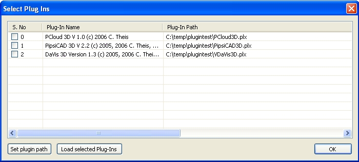
Figure 5: Plugin selection dialog.
The default plugin path, which will be used by SimpleGeo searching for plugins, can be set via the "Set plugin path" button. All plugins that were found in the currently set plugin path will be displayed with name and version information. In order to load them it is necessary to select them by clicking on the check box and pressing the "Load selected Plug-Ins" button. Subsequently, new buttons appear in the toolbar which will activate the respective plugin.
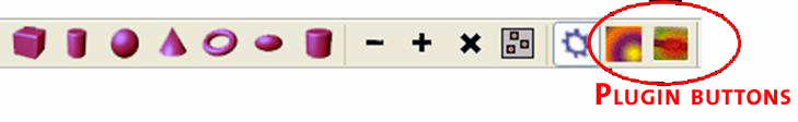
Figure 6: Toolbar with dynamicall added plugin buttons.
Unloading plugins |
Plugins can also be removed dynamically if this is required. The procedure is similar to loading by bringing up the plugin dialog via via the menu item Macros -> Load plugins. All currently active plugins are marked by check boxes. To unload these plugins click on the check boxes to deactivate them and click on the "Load selected Plug-Ins" button. Only those plugins which are still tagged by active check boxes will remain.
DaVis3D is a plugin which allows for superimposing data on top of the geometry. The data is expected to have the 3D structure of a cuboid (e.g. cartesian USRBIN in FLUKA or mesh tally in MCNPX), where each voxel (=small cube) has some value assigned to it. Up to three projection planes (XY, YZ, ZX) can be activated and moved through the dataset interactively. The results at the positions of the respective planes are displayed immediately. Starting from version 2.5 onwards it is possible to display several data sets at the same time. This is done by creating a copy of the VDaVis3D.plx file in the plugin-installation directory. As a consequence a second instance of the plugin can be loaded which can be used to display an additional data set which can have deviating topological properties (e.g. cylindrical binning) or a different mesh resolution.
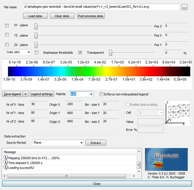
Figure 6: Main control dialog of DaVis3D.
File formats:
DaVis3D supports a number of different ASCII file formats for display. At the moment these are:
Post process data:
Starting with version 3.5 of DaVis3D it is possible to perform various post processing steps on FLUKA USRBIN files (cartesian, RZ, R-Phi-Z in ASCII format). The probably most important one is the calculation ov agerages + the associated error which will be explained below. Furthermore it is possible to calculate:
Please note that the original FLUKA USRBIN format is retained in the result files. Consequently, they can be used with whatever other program that is capable of reading FLUKA USRBIN files in ASCII format.
The default action is set to "data averaging" but any other post processing procedure can be selected by clicking on the down-arrow located at the right side of the "Average" button. This will open a menu from which the requested action can be selected.
Data averaging:
In order to facilitate the analysis of FLUKA files DaVis3D is capable of calculation the average + the statistical error of several USRBIN files. Pressing the "average" opens a dialog where the user can select a number of files that should be considered in the calculation of the mean. If the files were not created with the same weight they will be taken into account accordingly and the user will be notified. If requested this feature can be turned off via the respective check box in the dialog. The topological properties and the size of the data set are of no concern for the averaging!
Data display:
The user can select the data to be loaded either by typing in the full path manually or select it using the "..." button to open a file dialog. The data is finally loaded after clicking on the "Load data" button. Subsequently, a dialog will pop up which offers the possibility to normalize the loaded data using an arbitrary multiplicative normalization factor. After the data have been loaded the range of values that are displayed can be selected. By default the smallest and the largest value encountered in the dataset are suggested. In addition, the binning type (linear or logarithmic) can be chosen.
After this procedure the information about the number of bins, the spatial origin of the data, bin size etc. are displayed as well as the color lookup table (LUT). Please note that all values in the LUT indicate the lower bin limit! The respective data projection planes can be activated by clicking on the check boxes next to the slider controls. Using the sliders it is possible to interactively move the linked plane through the data set.
 |
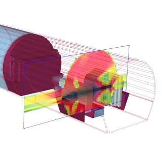 |
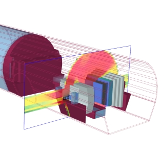
Figure 7: Displaying fluences with transparency but without "enforce overlay" (left), and with "enforce overlay" (right).
Rendering can be controlled by the user by setting the transparency via the provided slider as well as the "Enforce overlay" checkbox. By default all graphical objects are ordered with respect to their distance from the current viewpoint. Therefore, objects in front cover those in the back. As a consequence the geometry might cover the data planes, which might not be desired. Checking the enforce overlay box solves this problem by forcing the data to be displayed in front, regardless of its actual position in space (see Fig. 7). Another way to gain some "insight" is to set the X-ray mode for an object. As a consequent it will appear transparent and the data "inside" this object becomes visible. Please note that for this option to work correctly the data must not be made transparent!
The user can choose from 2 different rendering modes:
Color plot
Contour plot
Color plots are the "traditional" plots that show gradients nicely. A number of different configurations for the color lookup table is available from the "Palette" drop down box. If "contour plot" was selected only gradient lines from one color (value) to another are shown. Please note that for this options only 21 fixed colors are available to avoid confusion!
Hint: If it is desired to combine both rendering options the best effect can be achieved by the following trick.
Create a copy of the VDaVis3D.plx file
Load the original plugin & the copy at the same time (even more than 2 instances can be loaded)
Load the same data in both instances
In the first plugin "color plot" should be chosen whereas in the second "contour plot" should be selected
The transparency in the first "color plot" should be set to ~30 - 50%
Data extraction:
The user has the possibility to extract the data which is currently displayed. The following extraction options are supported:
It is possible to obtain the data of a plane as a 2D matrix by clicking on the "Extract" button while "Plane" is selected in the source drop-down box.
All values found at the intersection of two active planes can be extracted by selecting "profile" from the drop-down box. In succession a dialog will be opened which allows the user to specify the intersection of which planes should be considered. In this dialog there is also the option to directly plot the values along the intersection line.
The basic functionality is identical to the extraction of a standard profile (see above). However, several averaging bins can be selected perpendicular to the profile direction. In addition also the profile direction can be "shrunk" as averages over several bins are calculated.
For example the user wants to calculate the profile along a tunnel in Z direction which has a width of 100 cm (e.g. 10 bins) in Y and X direction. A standard profile of the intersecting planes XZ & YZ would yield the profile of 1 bin width (10cm) along the Z axis. An averaged profile however could yield a profile along the Z axis using X and Y values which have been averaged over the whole width of the tunnel. Naturally the number of bins used for averaging in the X direction could be different (e.g. 2 bins = 20 cm) from those defined for the Y direction. A detailed description is also given directly in the dialog where the settings can be made.
If all 3 planes are selected the intersection forms the center of an octant constituted by the neighboring bins. Choosing the "octant" as an extraction data source will write the exact values of these 8 bins as well as the average + error to a file.
See the paragraph data probing for a description of the definition of arbitrary averaging volumes. All values + the average and standard deviation are extracted and written to a file.
In case the resolution of the original data is too fine DaVis3D offers the functionality to rebin the data and export it in a native FLUKA USRBIN ASCII output format. The user will be prompted to input how many bins in each direction should be combined via averaging.
Data probing:
If all 3 planes are selected it is possible to retrieve the
exact data value of one of the 8 adjacent bins. From the drop-down box the user
can select which bin should be considered and this bin will be shown outlined as
a gray cube. Furthermore, the average of all 8 values can be calculated
automatically by selecting "Octant".
In addition from version 3.0 it is possible to define an arbitrary averaging
volume with the origin being at the intersection point of all 3 planes. After
selecting "Arbitrary avg." from the data probing list box a
configuration dialog is shown. In this dialog the user can enter the number of
voxels that will be considered for averaging in the
positive and negative direction of each axis! Moving the planes with this
option active will also move the defined averaging volume and the average will
be calculated on-the-fly. In order to extract the values and the associated
average + error please use the data extraction option.
Threshold detection:
This feature allows to emphasize thresholds in the color plot. Selecting this option will pop up a dialog asking for up to three specified thresholds. Subsequently, the algorithm will search for these thresholds and use a contour line to delimit areas above and below the specified values. As a consequence it is easier to find and emphasize limits even in very smoothly colored plots with a large number of colors.
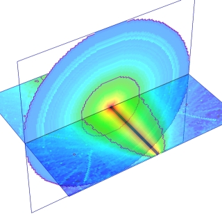
Figure 8: Threshold detection for a RZ plot. The actual threshold is indicated by the contour shown in violet.
General settings:
By clicking with the right mouse button on the DaVis3D label in the taskbar the system menu opens which offers the "Settings" item. On one hand the user can turn off the blue borders showing the plane limits and on the other hand a transformation matrix can be defined for the visualization. FLUKA for example by now offers the possibility to define transformation matrices which are applied to USRBIN scorings. However, the created output files contain the information of the scoring location without the transformation matrix being applied! The header only includes a message that a transformation matrix with index # has been applied. As the file is lacking the actual information about the matrix parameters (translation & rotation) the plot can only be done using the non-transformed spatial information which is available in the file. In order to plot the data correctly at the position of scoring one has to look up the transformation parameters that were defined in FLUKA and enter them manually in the settings dialog.
Another option provided by the general settings is the format of the legend which can be change into "superscript" mode instead of scientific E notation.
Colors & color bar:
By default 21 colors are used but a larger number of colors can be selected to obtain smoother plots. Starting with version 2.5 the palette will be interpolated if a larger number than 21 is chosen. However, the user can still revert to a block-type non interpolated legend by ticking the "enforce non interpolated legend" check-box.
A standard palette is provided but the users can supply their own color schemes by preparing a simple ASCII file:
The file is a simple ASCII file with the following format:
Please note that only an arbitrary number of fixed color points must be supplied as all color values in between are automatically interpolated.
For example the following file will give you a LUT with 256 colors ranging from white to black.
# ColorLUT 1.0
0, 1.0, 1.0, 1.0
255, 0.0, 0.0, 0.0
Another example:
# ColorLUT 1.0
0, 1.0, 1.0, 1.0
64, 0.0, 0.0, 1.0
128, 0.0, 1.0, 0.0
196, 1.0, 0.0, 0.0
255, 0.0, 0.0, 0.0
XYZ-ASCII file format:
The XYZ ASCII format is a very simple file based on a cuboid voxel description. It includes a header of 6 lines which is mandatory and includes the information about the spatial extension (X-start, X-end, etc...) and the number of bins in X,Y,Z. An example is:
VOXEL-DATA @2003 MEULLER-THEIS
X-start: 1820 X-end: 2080 X-steps: 13
Y-start: -2500 Y-end: -500 Y-steps: 100
Z-start: -1200 Z-end: 1200 Z-steps: 120
===========================================
X Y Z Data
Following this the data are given in four rows. The first three rows indicate the voxel index (X,Y,Z) and the fourth represents the actual data value. Each voxel can be imagined as a small cube with a value associated to it. For the aforementioned example header the index in X would run from 0 to 12, the Y index from 0 to 99, and the Z index from 0 to 119, with X incrementing fastest!
For example:
0 0 0 4.25180000e-04
1 0 0 5.28470000e-04
2 0 0 8.84020000e-04
3 0 0 2.84720000e-04
4 0 0 2.46480000e-04
5 0 0 2.80910000e-04
A full example would look like the following:
VOXEL-DATA @2003 MEULLER-THEIS
X-start: 1820 X-end: 2080 X-steps: 13
Y-start: -2500 Y-end: -500 Y-steps: 100
Z-start: -1200 Z-end: 1200 Z-steps: 120
===========================================
X Y Z Data
0 0 0 4.25180000e-04
1 0 0 5.28470000e-04
2 0 0 8.84020000e-04
3 0 0 2.84720000e-04
4 0 0 2.46480000e-04
5 0 0 2.80910000e-04
6 0 0 5.36890000e-04
7 0 0 4.44160000e-04
8 0 0 7.55120000e-04
9 0 0 1.86970000e-04
10 0 0 9.13150000e-05
11 0 0 2.14480000e-04
12 0 0 4.15230000e-04
0 1 0 5.16390000e-04
1 1 0 1.08070000e-03
2 1 0 5.15360000e-04
3 1 0 6.56130000e-04
4 1 0 6.30410000e-04
5 1 0 3.88420000e-04
6 1 0 4.84400000e-04
7 1 0 8.01480000e-04
8 1 0 3.57960000e-04
9 1 0 8.01870000e-05
10 1 0 4.36080000e-04
11 1 0 5.80280000e-04
12 1 0 2.14270000e-04
0 2 0 1.01640000e-03
1 2 0 7.64250000e-04
2 2 0 3.06020000e-04
......
PCloud3D is a plugin which helps to visualize particle positions and their directions. Optionally, the results can be displayed with the geometry which is very helpful if one wants to check the results of sampled starting positions for particles. All particles are color coded which can be configured by the user and a filter for certain particle types can be applied. Furthermore, some statistical information about the particle energies, particle types and also a combination of these two quantities is available.
Data format:
* Native ASCII format which is explained below
* MCNPX output files (table 150) can be read directly to visualize the source
particles.
NATIVE PCloud3D-ASCII file format:
The native PCloud3D ASCII file is very simple with each line marking one particle position and direction. It's a column oriented format but there are no alignment or any other formatting restrictions.
Particle-Number Weight PositionX PositionY PositionZ DirectionX DirectionY DirectionZ Energy
For example:
8 0.10E+01 -0.17624E+03 -0.15900E+04 0.87634E+03 -0.23013E-01
-0.78658E+00 0.61706E+00 0.25090E+00
8 0.10E+01 -0.23553E+03 -0.15900E+04 -0.65244E+00 0.15487E+00 -0.97602E+00 0.15299E+00
0.29711E-01
8 0.10E+01 -0.38518E+03 -0.15900E+04 -0.81991E+03 -0.22731E+00 -0.91131E+00 -0.34329E+00
0.12879E-07
8 0.10E+01 0.61460E+02 -0.15900E+04 -0.52722E+03 0.84339E-01 -0.89318E+00 -0.44172E+00
0.10219E-02
8 0.10E+01 0.11239E+04 -0.15900E+04 -0.24981E+03 0.57786E+00 -0.81366E+00 0.63563E-01
0.16738E-01
8 0.10E+01 0.86034E+02 -0.15900E+04 -0.17400E+03 0.38581E-01 -0.97904E+00 -0.19996E+00
0.11648E-02
Please note that the particle number is corresponding to the numbers used by FLUKA! The MCNPX importer handles the transformation of the numbering scheme automatically!
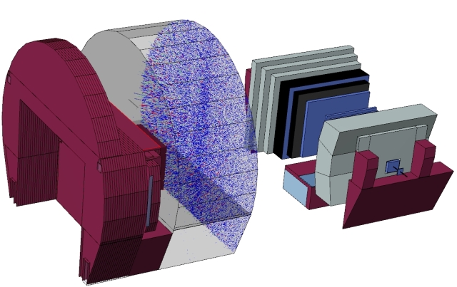
Figure 9: Particle stopped in air after a beam loss simulation at CERN's LHCb detector. The position as well as the direction is shown with the direction arrows being scaled according to the particle energy
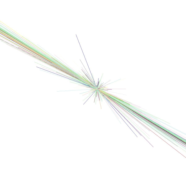
Figure 10: Calculation of p-p collisions at 7 TeV. The results were done with DPMJET3 (author S. Roesler) for which an interface was implemented to extract the required information.
Description
PipsiCAD3D is a toolkit which couples SimpleGeo and FLUKA to display particle
tracks in 3D, superimposed
on top of the geometry. Particle tracks can be visualized statically, in terms
of all tracks being
displayed at once, or they can be animated as a function of time. Consequently,
the temporal evolution of
showers and tracks can be studied. Due to the time information obtained from
FLUKA the relative speed
of the particles with respect to each other is correct and thus, fast neutrons,
for example, will be
animated considerably faster than slow neutrons.
All particle types are color coded which can be configured by the user. Furthermore,
it is possible to
apply filters with respect to the track segment energy, as the first (!) filter
criterion, and the particle
type, as the second (!) filter criterion.
HOW TO USE IT
The first step is to set up a FLUKA simulation which produces a collision
tape by inserting a
USERDUMP statement:
USERDUMP 100. 30. 6.0 collcad
(What1 = 100, WHAT2 = 30, WHAT 3 = 6.0, SDUM = collcad)
Please
see the FLUKA manual for a detailed description of the USERDUMP parameters.
The standard FLUKA collision tape does not contain temporal information and
thus, it is necessary
to compile and link FLUKA with a proprietary mgdraw.f routine
which ships with this plugin package.
The next step is to run the linux interface
named pipsicad_simplegeo to process the binary collision tape.
During this preprocessing minimum and maximum energy thresholds can be applied
and the number of
energy bins and the binning type (linear or logarithmic) is selected. The result
is an ASCII file
which can be loaded by the PipsiCAD3D.plx
plugin in SimpleGeo.
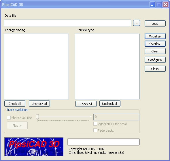
Figure 11: Main control dialog of PipisCAD3D.
After loading the data all tracks can be displayed
statically by selection the "Visualize" button
in
the PipsiCAD3D main dialog (see Figure 10) . Ticking the "Show evolution" check
box will enable a
slider that can be used
to show the tracks at a certain time. By default the start and the end time
are taken corresponding to
the minimum and maximum values that were found in the data.
Depending on
the problem set it might
be preferable if the time steps are increased not linearly but
logarithmically
which can be done
by ticking the respective check box in the dialog.
Once a track is drawn it does not vanish or fade but remains visible throughout
the rest of the
animation. If this behavior is not desired it is possible to fade tracks that
exceed a certain number
of time steps after they have terminated. Please note that fading is available
for a linear time scale!
All settings, like the absolute start time and end time of the temporal period
to be studied, the
total length of the animation etc. can be defined via the "Configure" dialog.
Please note that the
total length of animation that is specified could be exceeded as your operating
system is not a
realtime OS and thus, some time might be dedicated to other tasks while showing
the animation!!
!!!!!!!!!!!!!!!!!!!!!!!!!!!!!!!!!!!!!!!!!!!!!!!!!!!!!!!!!!!!!!!!!!!!!!!!!!!!!!!!!!!!!!!!!!!!!!!!!!!!!!!
!! IMPORTANT: Please note that depending on the problem set collision tapes
can
!! be VERY VERY big, especially if the electromagnetic cascade is taken
!! into account. Thus, it is recommended to start with a low number of
!! source particles (e.g. 1!).
!!!!!!!!!!!!!!!!!!!!!!!!!!!!!!!!!!!!!!!!!!!!!!!!!!!!!!!!!!!!!!!!!!!!!!!!!!!!!!!!!!!!!!!!!!!!!!!!!!!!!!!
HINT:
By default the user can select an energy bin as the first
filter criterion for visibility, and the particle type
as the second filter criterion. However, sometimes it might be interesting
to perform a selection by
particle type
only, regardless of the energy. This can be done by creating one energy bin
only and thus,
the particle
type selection will be applied to all energies within the minimum and maximum
energy that
was specified.
SHORT SUMMARY
1.) Compile and link the proprietary mgdraw.f to FLUKA
2.) Add a USERDUMP statement to your input to produce a collision tape
3.) Run your simulation to create a collision tape
4.) Run the linux interface to select the energy range & binning of the
particles that will be extracted
5.) Load your geometry and the PipsiCAD3D plugin in SimpleGeo
6.) Load the created data file with the plugin and press the "Visualize" button
7.) Optionally, you might select track evolution display and animate the resulting
tracks
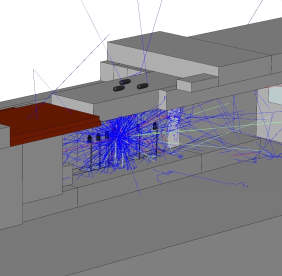
Figure 12: Example of the hadronic cascade caused by 1 proton of 120 Gev/c impinging on a copper target at the CERF facility.
Loading/Importing/Exporting
1.1 FLUKA importer: "Problem with line: ... ARB, RAW, WED not implemented" |
The bodies ARB, RAW and WED have not been implemented in SimpleGeo. The user is encouraged to replace them using other bodies like planes for example.
1.2 FLUKA importer: "Unrecognizable input: ..." |
SimpleGeo's parser is much more flexible than FORTRAN's fixed format which delimits lines in fixed columns. However, for the parser to be able to recognize different entities (tokens) it is important that a delimiter is supplied. In view of FLUKA's new free format the user should delimit different tokens by a space, a comma or a semicolon. In some fixed format input files two tokens are not delimited and thus, cannot be recognized separately by SimpleGeo. If such a problem appears one should search the specified line in the input file and separate the different tokens by a space. Under Windows a tool is available (AlignmentFix) which will automatically perform this procedure. Please contact the author to get a recent copy.
1.3 FLUKA importer: "ATTENTION: No source primitive ... was found while trying to build the CSG tree" |
This error message can be triggered by two causes. Either you have not supplied the geometry description of the mentioned primitive or the name (number) of the primitive did not EXACTLY match the one you used in the region description. Please note that the importer is already oriented towards string literals (names) as body identifiers. Thus leading zeros are not dropped and a body ID of 003 DOES NOT EQUAL 3!! In order to avoid such problems it is strongly suggested not to use any leading zeros as body IDs!!
1.4 FLUKA importer: "Number of material assignments did not match the number of regions" |
You either assigned materials to regions that do not exist (anymore) or you are lacking material assignments. Please check your FLUKA input and keep in mind that FLUKA's material assignment parameter indicates the number of the region (= the position in the input file!!!) not not the region ID that you have assigned.
1.5 ALIFE importer: "Number of material assignments did not match the number of regions" |
You probably introduced comments within a region description. Please keep in mind that for one region which might consist of several sub-regions that are linked by a union, all the lines forming this region must be consecutive without any blank line or comment in between!
1.6 FLUKA importer: "I try to open a file which makes use of the new syntax but it doesn't work" |
Are you sure that you have selected the correct import filter? Please keep in mind that files using names instead of numbers and must show the extension ".new.inp"!
1.7 Can I load & visualize LATTICE geometries? |
Starting with version 4.x SimpleGeo supports lattice geometries. However, there are some constraints imposed by the different approaches of the various Monte Carlo codes which the user should be aware of.
FLUKA:
Due to the approach adopted by FLUKA interactive visualization of
lattice regions is not possible. Commonly, lattice geometries are implemented by
associating a transformation matrix with a source region that is to be
replicated. In that case the information on the intrinsic properties of the
source is available and a copy can be visualized at arbitrary positions without
requiring additional regions or primitives. In FLUKA the inverse approach has
been implemented which requires the implementation of a container body (e.g., a
box) and a matrix which transforms this container back to an arbitrary sub-space
within the geometry. Any particle entering the container is transformed via the
given matrix and then tracked at the location obtained after the transformation.
As a consequence no real information about the source region is available but
the container primitive. As a consequence only container primitives can and will
be visualized interactively in SimpleGeo.
For the creation of lattice or rather replicated geometry objects in SimpleGeo please refer to the section "creation of replicas" in the manual.
MCNP(X): not yet implemented
PHITS: not yet implemented
1.8 I can load a file but SG crashes after I start the build process |
Please refer to section 3.4
1.9 Can I increase the number of digits that are used to export the parameters of bodies? |
Internally SimpleGeo stores values and performs the calculations with 15 significant digits. However, by default only 2 decimal digits are shown which is sufficient for most cases. With the exception of a number of special bodies that are prone to require a higher number of significant digits (e.g. rotated planes) the identical number of digits will be exported to FLUKA/MCNP(X) etc. In case more digits are required by the user in order to input parameters with the requested accuracy it is possible to increase this number via the options dialog that is available via "View" -> "Settings" -> "Nr. of property digits". This will increase the number of digits shown in the property view as well as those that are exported to any supported Monte Carlo transport code.
Visualization
2.1 After loading a file I can only see the graticule and a lot of colored areas |
After loading a file the standard projection is still applied. In
order to update the projection values to show the whole scenery the user has
to press the reset zoom button ![]() on
the toolbar once. This is required only once after the loading of the file
to update and activate the display caching system.
on
the toolbar once. This is required only once after the loading of the file
to update and activate the display caching system.
2.2 After loading a file I only a big gray box/sphere/... |
In contrast to "ordinary" CAD sketches and drawings your CSG geometry has to include all volumes like the surrounding blackhole or air-volumes. In order to obtain an image which is easier to understand one should consider turning off the visibility of blackhole, air and earth regions. (See section 2.9)
2.3 Some bodies are open/some bodies seem to have missing surfaces |
SimpleGeo is a hybrid-modeling system which converts analytical CSG bodies to approximated surface models (B-reps). This allows for rapid visualization using off-the-shelf hardware instead of expensive special purpose graphics boards. However, this approach sometimes suffers from floating point inaccuracy. A quite sophisticated error and margin handling system is implemented in SimpleGeo but pathological cases still can cause trouble. For example the result can be ambiguous if two faces of different primitives are coplanar. Unfortunately the ongoing research in this area of computer graphics and mathematics has not yet been able to devise a solution applicable to all cases.
One can try to solve these artefacts by changing for example the number of faces used to create curved surfaces of the affected primitives. Another "global" solution would be to change the values for the error margins under the global settings. However, this is only recommended for experienced users!!
It should be noted that visualization artefacts DO NOT have any influence on the exported model for the Monte Carlo codes, because the export filter operates on analytical descriptions, whereas the approximated models are used for visualization only.
Further information can be found in SimpleGeo's reference publication "Interactive three dimensional visualization and creation of geometries for Monte Carlo calculations", which will be published in the proceedings edition of Nuclear Instruments and Matter for AccApp05.
2.4 There are some faces of a cylinder protruding where they shouldn't |
As already indicated in section 2.3 B-reps suffer from floating point inaccuracies. Well, there is no such thing as a free lunch, but on the other hand they allow you to obtain interactive visualization without special purpose hardware. It has been noticed that B-rep kernels are in some situations sensitive to the order of the primitives used within a boolean operation. From a mathematical point of view the intersection of A & B & C is equal to the intersection of B & A & C. However, this does not necessarily hold true using floating point calculations, especially if one or more primitives are planes. The importer of SimpleGeo includes an algorithm which performs a pre-sort to exclude most of the problematic cases but sometimes this general approach does not work. Another complication are the use of infinite planes. Infinity is simply not possible to model with a computer that has limited accuracy. Therefore, infinity has been assigned a fixed value, which is appropriate for most but not for all cases.
There are basically two things that you can do:
A.) Try to change the setting for infinity to a smaller (or larger) value in the "View"-"Settings" dialog. Consequently enforce a rebuild of the geometry pressing Ctrl+R. Keep in mind that the current settings of infinity are saved together with the geometry.
B.) Try to change the order of the respective
nodes:
In this case the user can change the order
of the primitives used in an boolean operation by just selecting one primitive,
dragging it over its parenting boolean
operator and dropping it there. Consequently, the primitive will be re-inserted
at the end of the boolean's child primitives. This process can sometimes
require a little playing around and testing until the required result is achieved.
There are a couple of guidelines which one can follow:
1.) In an intersection the plane intersecting for example infinite cylinders should come before the cylinder
2.) In a difference the plane being subtracted from an infinite cylinder should come after the cylinder
Due to the hybrid-nature of the modeler these artefacts DO NOT have any influence on the exported model for the Monte Carlo codes. Hence, if one does not want or have time to fix these artefacts the visibility of the region can simply be turned off.
2.5 When I select an item in the tree it takes quite long until its properties appear and its outline is highlighted in red |
This is clearly an indication that your graphics card is reaching its limit. If you resort to a non-shaded rendering (e.g., sketch rendering) you will notice that this resolves this problem. In this case you should only go back to a shaded rendering if it is really necessary.
2.6 I would like to see inside my geometry |
There are actually several ways to achieve this. You could either change the transparency setting of the respective material or you could simply use one of the available additional rendering modes. By default a flat shaded rendering is performed and thus only the outer faces of opaque objects are visible. However, by chosing the "Overlay sketch" rendering mode it is possible to "look inside". Just try it out and you will see that overlay sketch will emphasize the contours of all objects regardless of fact whether they are visible from the current point of view or not. Consequently, you will be able to peek inside bounding volumes.
2.7 The debugger has found errors in my geometry and I've clicked on visualize. However, I don't see them |
Please read the hint in the debugging section.
2.8 Turning on and off the visibility of the same regions manually is very cumbersome. Can I save the visibility state? |
Yes you can. For a description please refer to the "Layers
& Visibility" section in the manual. You should just be aware that The visibility
state is saved as a kind of visibility image of the CSG tree. Whenever you
change the order of the child-nodes of the root node, this will not be taken
into account by a previously saved snapshot. This means that for example node
number 3 is invisible and node number 4 is visible at the time of creating
the snapshot. At some point you might swap the nodes and the old node number
3 becomes node number 4 and vice versa. Applying the previously saved snapshot
will render node number 3 invisible and node number 4 visible, no matter which
object is placed there. However, it does not matter if you add new nodes at
the end of the CSG tree, which is the default behavior. They are not affected
by loading an old snapshot.
2.9 Can I turn off all regions with a specific material assignment at once? |
Yes, you can. If you take a look at the screen you will
see the CSG tree on the left. Below the tree you will find two tabs ![]() .
By default the CSG tree tab is activated but you can klick on the "Materials"
tab to obtain a list of all materials in the current scenery. By clicking on
the light bulb or double clicking on the material name you can turn off the
visibility of all regions sharing that specific material assignment.
.
By default the CSG tree tab is activated but you can klick on the "Materials"
tab to obtain a list of all materials in the current scenery. By clicking on
the light bulb or double clicking on the material name you can turn off the
visibility of all regions sharing that specific material assignment.
Visualization & Construction
3.1 I've loaded a file but when I turn on the building of the geometry it takes ages... |
Building the geometry can be quite a CPU challenging task, whereas the visualization is a GPU demanding task. This means that even the fastest graphics card won't help you during the first build of the geometry. SimpleGeo utilizes a geometry caching system which can only kick-in after the first build of the scenery is performed. Therefore, a longer waiting time is to be expected at the beginning.
The more curved surfaces you have in your geometry the longer it might take. For a start you can reduce the level of detail (LOD) via the built-in scripts to get an idea what the geometry looks like. In addition, you might consider turning off regions that you do not want to see anyway (black-hole, air, earth) before you turn on the building of the geometry via the automatic update button. As a consequence only regions set to visible will be created. By turning on the visibility of previously invisible regions the respective geometry will be created on demand.
3.2 If I click on an object for identification the response is rather slow... |
It was found that this is slow-down is due to some problems found with older ATI graphics drivers. Updating to Catalyst version >= 8.5 should resolve this problem.
3.3 Can I visualize LATTICE geometries? |
Please refer to section 1.7.
3.4 I can load a file but SG crashes after I start the build process |
For visualization SimpleGeo automatically transforms the analytical CSG description into a boundary representation via partitioning. If the imported CSG description lacks accuracy (e.g. rotated planes are not specified with the number of required digits etc.) or in case of rounding issues SimpleGeo tries to recover the situation which usually works at least to the point that only visualization artefacts should occur. However, we have seen one case where the resulting geometry was degenerated to a point that the recovery algorithms failed due to the significant lack of accuracy in the input model and SimpleGeo crashed while trying to build (= partition) the model. This problem can be circumvented by relaxing the constraints upon which the CSG kernel acts and performs the partitioning. The following steps are necessary for this:
Import of the geometry without clicking on the "automatic build" gearwheel button!
Open the settings dialog via the menu item "View" --> "Settings"
Modification of the "Minimum vertex tolerance" setting in the CSG kernel settings. By default this value is 1E-3. As a starting point one can use 1E-2 or 1E-1 and choose "relaxed" as the setting for the vertex comparison accuracy.
This workaround should be sufficient to allow for visualizing the geometry. However, one should not forget that the original model still lacks accuracy and this is where the actual problem originates! Relaxing the accuracy constraints should only be considered as a temporary work-around! Eventually the source geometry should be provided with the required accuracy as the lack of accuracy indicates that there could be also problems in the tracking phase during transport calculations!
Debugging
4.1 FLUKA crashes but SimpleGeo's debugger reports no error |
In general it is important to keep in mind that the absence
of errors in the debugger does not guarantee the absence of errors in the
geometry. It could have been the case that the settings used for the debugging
(e.g., which regions were debugged, which debugging resolution: grid resolution
or total number of points) were not appropriate to find small scale errors.
However, if FLUKA crashes with an error like: "Exit being called from
G1, next region not found" one of the following two points could be the
reason:
There is an overlap of an infinite body with the blackhole which should be the outermost body.
The geometry was constructed using recursive structures which imply the use of parentheses. However, for exporting only the new syntax (file suffix: .new.inp) was selected instead of new syntax with parentheses (file suffix: .par.inp)!
General topics
5.1 What are all these "autosave" and "bak" files about? |
Please see the section about Auto-Save and backup for a detailed explanation.
5.2 I get a "cannot create default material database" message when starting the program |
By default the program tries to establish a "default material database" in the installation directory. In case you are running under Windows Vista you might lack the user privileges to write to directories under the "Program Files" directory structure. As a remedy you might disable the user account control of Windows Vista or grant your user account the necessary privileges.
(See: http://blogs.msdn.com/uac/archive/2006/01/22/516066.aspx)
5.3 I've loaded the plugins but I cannot see their icon on the toolbar |
With Windows Vista Microsoft introduced new toolbars which are now also available under Windows XP. Due to some changes the plugin mechanism had to be adapted and as a consequence the plugins will show up with their name instead of an icon!
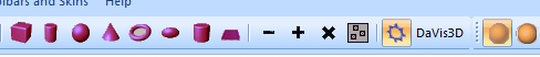
However, if the toolbar determines that there is not enough space to show the new button it will draw a small arrow at the right side. Once the user clicks on this arrow a drop down box will appear which contains all toolbar buttons that were not yet shown due to space restrictions.
5.4 I've installed the plugins & set the plugin path correctly but I still get the message "ERROR: No Plug-Ins found" |
With Microsoft's introduction of the side-by-side & manifest mechanism, which allows for hosting various versions of the runtime libraries at the same time, there have been some rare cases of version mix-ups on some machines. Consequently, the plugin mechanism wasn't able to determine and correctly locate the required runtime libraries and therefore the plugins could not be loaded. To circumvent this problem a fresh installation of the VC++ runtime components is required:
SimpleGeo's installation package contains a folder labelled "vcredist_x86" which contains a program named "vcredist_x86.exe". This package will install the latest version of the runtime components and set up the operating system accordingly.
5.5 Can I increase the number of digits that are shown in the properties? |
Please refer to section 1.9
5.6 Upon opening the "load plugins" dialog one or more of the plugins does not show up |
Please refer to FAQ 5.4. You might need to update your operating system libraries.
5.7 I cannot send e-mails but receive a "Mail system cannot be invoked via the operating system" message |
This issue might show up in Windows Vista or later as a side-effect of the more restrict user account control. In order to invoke a different process, like the mailing system in this case, the caller as well as the called program need to run with the same permission level. For example if SimpleGeo is executed with administrator rights then also your mail program should be run with administrator rights. In case the execution level of the called program is lower then the call will be blocked! Please check that both programs are run with at the same security level. More info can be found at: http://technet.microsoft.com/en-us/library/cc709628(WS.10).aspx and http://technet.microsoft.com/en-us/windows/dd572175.aspx
|
Theis C., Buchegger K.H., Brugger M., Forkel-Wirth D., Roesler S., Vincke
H.,
"
Interactive three dimensional visualization and creation of geometries for
Monte Carlo calculations",
Nuclear Instruments and Methods in Physics Research A 562, pp. 827-829 (2006).